Polynomial Regression From Scratch With PyTorch

Create the polynomial features

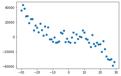
The formula of linear regression is as follow: \[\begin{align} \boldsymbol{\hat{y}} = \boldsymbol{X}\boldsymbol{w} \end{align}\] where \(\boldsymbol{\hat{y}}\) is the target, \(\boldsymbol{w}\) are the weights learned by the model and \(\boldsymbol{X}\) is training data. Polynomial regression is still considered as a linear regression because there is only linear learning parameters: \[\begin{align} \boldsymbol{y} = \boldsymbol{w}_0 + \boldsymbol{X}\boldsymbol{w}_1 + \dots + \boldsymbol{X}^n\boldsymbol{w}_n \end{align}\] As you have probably guessed, this equation is not linear. We use a trick to make it linear:

• We gather all the \(\boldsymbol{X}^2\) to \(\boldsymbol{X}^n\) as new features that we created and we concatenate them to \(\boldsymbol{X}\).
• All the \(\boldsymbol{w}_1\) to \(\boldsymbol{w}_n\) are concatenated to \(\boldsymbol{w}_0\).

At the end, the polynomial regression has the same formula as the linear regression but with the aggregated arrays.

def create_features(X, degree=2, standardize=True):
    """Creates the polynomial features
    
    Args:
        X: A torch tensor for the data.
        degree: A intege for the degree of the generated polynomial function.
        standardize: A boolean for scaling the data or not.
    """
    if len(X.shape) == 1:
        X = X.unsqueeze(1)
    # Concatenate a column of ones to has the bias in X
    ones_col = torch.ones((X.shape[0], 1), dtype=torch.float32)
    X_d = torch.cat([ones_col, X], axis=1)
    for i in range(1, degree):
        X_pow = X.pow(i + 1)
        # If we use the gradient descent method, we need to
        # standardize the features to avoid exploding gradients
        if standardize:
            X_pow -= X_pow.mean()
            std = X_pow.std()
            if std != 0:
                X_pow /= std
        X_d = torch.cat([X_d, X_pow], axis=1)
    return X_d

def predict(features, weights):
    return features.mm(weights)

features = create_features(X, degree=3, standardize=False)
y_true = y.unsqueeze(1)

Method 1: Normal equation

The first method is analytical and uses the normal equation. Training a linear model using least square regression is equivalent to minimize the mean squared error:

\[\begin{align} \text{Mse}(\hat{y}, y) &= \frac{1}{n}\sum_{i=1}^{n}{||\hat{y}_i - y_i ||_{2}^{2}} \\ \text{Mse}(\hat{y}, y) &= \frac{1}{n}||\boldsymbol{X}\boldsymbol{w} - \boldsymbol{y} ||_2^2 \end{align}\]

where \(n\) is the number of samples, \(\hat{y}\) is the predicted value of the model and \(y\) is the true target. The prediction \(\hat{y}\) is obtained by matrix multiplication between the input \(\boldsymbol{X}\) and the weights of the model \(\boldsymbol{w}\).

Minimizing the \(\text{Mse}\) can be achieved by solving the gradient of this equation equals to zero in regards to the weights \(\boldsymbol{w}\):

\[\begin{align} \nabla_{\boldsymbol{w}}\text{Mse}(\hat{y}, y) &= 0 \\ (\boldsymbol{X}^\top \boldsymbol{X})^{-1}\boldsymbol{X}^\top \boldsymbol{y} &= \boldsymbol{w} \end{align}\]

For more information on how to find \(\boldsymbol{w}\) please visit the section “Linear Least Squares” of this link.

def normal_equation(y_true, X):
    """Computes the normal equation
    
    Args:
        y_true: A torch tensor for the labels.
        X: A torch tensor for the data.
    """
    XTX_inv = (X.T.mm(X)).inverse()
    XTy = X.T.mm(y_true)
    weights = XTX_inv.mm(XTy)
    return weights

weights = normal_equation(y_true, features)
y_pred = predict(features, weights)

plt.scatter(X, y)
plt.plot(X, y_pred, c='red')

With the normal equation method, the polynomial regressor fits well the synthetic data.

Method 2: Gradient Descent

The Gradient descent method takes steps proportional to the negative of the gradient of a function at a given point, in order to iteratively minimize the objective function. The gradient generalizes the notion of derivative to the case where the derivative is with respect to a vector: the gradient of \(f\) is the vector containing all of the partial derivatives, denoted \(\nabla_{\boldsymbol{x}}f(\boldsymbol{x})\).

The directional derivative in direction \(\boldsymbol{u}\) (a unit vector) is the slope of the function \(f\) in direction \(\boldsymbol{u}\). In other words, the directional derivative is the derivative of the function \(f(\boldsymbol{x} + \sigma \boldsymbol{u})\) with respect to \(\sigma\) close to 0. To minimize \(f\), we would like to find the direction in which \(f\) decreases the fastest. We can do this using the directional derivative:

\[\begin{align} &\min_{\boldsymbol{u}, \boldsymbol{u}^\top \boldsymbol{u} = 1}{\boldsymbol{u}^\top \nabla_{\boldsymbol{x}} f(\boldsymbol{x})} \\ = &\min_{\boldsymbol{u}, \boldsymbol{u}^\top \boldsymbol{u} = 1}{||\boldsymbol{u}||_2 ||\nabla_{\boldsymbol{x}}f(\boldsymbol{x})||_2 \cos \theta} \end{align}\]

ignoring factors that do not depend on \(\boldsymbol{u}\), this simplifies to \(\min_{u}{\cos \theta}\). This is minimized when \(\boldsymbol{u}\) points in the opposite direction as the gradient. Each step of the gradient descent method proposes a new points: \[\begin{align} \boldsymbol{x'} = \boldsymbol{x} - \epsilon \nabla_{\boldsymbol{x}}f(\boldsymbol{x}) \end{align}\]

where \(\epsilon\) is the learning rate. In the context of polynomial regression, the gradient descent is as follow: \[\begin{align} \boldsymbol{w} = \boldsymbol{w} - \epsilon \nabla_{\boldsymbol{w}}\text{MSE} \end{align}\] where: \[\begin{align} \nabla_{\boldsymbol{w}}\text{MSE} &= \nabla_{\boldsymbol{w}}\left(\frac{1}{n}{||\boldsymbol{X}\boldsymbol{w} - \boldsymbol{y} ||_2^2}\right) \\ &= \frac{2}{N}\boldsymbol{X}^\top(\boldsymbol{X}\boldsymbol{w} - \boldsymbol{y}) \end{align}\]

def gradient_descent(X, y_true, lr=0.001, it=30000):
    """Computes the gradient descent
    
    Args:
        X: A torch tensor for the data.
        y_true: A torch tensor for the labels.
        lr: A scalar for the learning rate.
        it: A scalar for the number of iteration
            or number of gradient descent steps.
    """
    weights_gd = torch.ones((X.shape[1], 1))
    n = X.shape[0]
    fact = 2 / n
    for _ in range(it):
        y_pred = predict(X, weights_gd)
        grad = fact * X.T.mm(y_pred - y_true)
        weights_gd -= lr * grad
    return weights_gd

features = create_features(X, degree=3, standardize=True)
weights_gd = gradient_descent(features, y_true)

pred_gd = predict(features, weights_gd)

The mean squared error is even lower when using gradient descent.

plt.scatter(X, y)
plt.plot(X, pred_gd, c='red')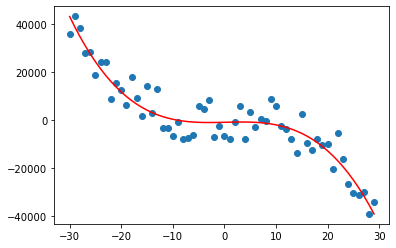

Conclusion

The polynomial regression is an appropriate example to learn more about the concept of normal equation and gradient descent. This method work well with data that has polynomial shapes but we need to choose the right polynomial degree for a good bias/variance trade-off. However, the polynomial regression method has an important drawback. In fact, it is necessary to transform the data to a higher dimensional space which can be unfeasable if the data is very large.

Can’t stop learning ? Read the next article of this series on Naive Bayes Classifier.