In this experiment, the Naive Bayes Classifier method will be implemented from scratch using PyTorch. We will train our model on the Student Alcohol Consumption dataset to try to predict if a student frequently drink alcohol or not.
Before starting, feel free to read the previous article of this series.
The data contains the following attributes:
school: student’s school (binary: ‘GP’ - Gabriel Pereira or ‘MS’ - Mousinho da Silveira)
sex: student’s sex (binary: ‘F’ - female or ‘M’ - male)
age: student’s age (numeric: from 15 to 22)
address: student’s home address type (binary: ‘U’ - urban or ‘R’ - rural)
famsize: family size (binary: ‘LE3’ - less or equal to 3 or ‘GT3’ - greater than 3)
Pstatus: parent’s cohabitation status (binary: ‘T’ - living together or ‘A’ - apart)
Mjob: mother’s job (nominal: ‘teacher’, ‘health’ care related, civil ‘services’ (e.g. administrative or police), ‘at_home’ or ‘other’)
Fjob: father’s job (nominal: ‘teacher’, ‘health’ care related, civil ‘services’ (e.g. administrative or police), ‘at_home’ or ‘other’)
reason - reason to choose this school (nominal: close to ‘home’, school ‘reputation’, ‘course’ preference or ‘other’)
guardian: student’s guardian (nominal: ‘mother’, ‘father’ or ‘other’)
traveltime: home to school travel time (numeric: 1 - 1 hour)
studytime: weekly study time (numeric: 1 - 10 hours)
failures: number of past class failures (numeric: n if 1<=n<3, else 4)
schoolsup: extra educational support (binary: yes or no)
famsup: family educational support (binary: yes or no)
paid: extra paid classes within the course subject (Math or Portuguese) (binary: yes or no)
activities: extra-curricular activities (binary: yes or no)
nursery: attended nursery school (binary: yes or no)
higher: wants to take higher education (binary: yes or no)
internet: Internet access at home (binary: yes or no)
romantic: with a romantic relationship (binary: yes or no)
famrel: quality of family relationships (numeric: from 1 - very bad to 5 - excellent)
freetime: free time after school (numeric: from 1 - very low to 5 - very high)
goout: going out with friends (numeric: from 1 - very low to 5 - very high)
health: current health status (numeric: from 1 - very bad to 5 - very good)
absences: number of school absences (numeric: from 0 to 93)
G1: first period grade (numeric: from 0 to 20)
G2: second period grade (numeric: from 0 to 20)
G3: final grade (numeric: from 0 to 20, output target)
Dalc: workday alcohol consumption (numeric: from 1 - very low to 5 - very high)
Walc: weekend alcohol consumption (numeric: from 1 - very low to 5 - very high)
import osimport mathimport torchimport numpy as npimport pandas as pdimport seaborn as snsimport matplotlib.pyplot as pltfrom pprint import pprintfrom sklearn.base import BaseEstimatorfrom sklearn.preprocessing import LabelEncoderfrom sklearn.model_selection import cross_val_score
Data Preparation
First, let’s read the data from .csv files and merge them together:
students_mat = pd.read_csv(os.path.join('data', 'student-mat.csv'))students_por = pd.read_csv(os.path.join('data', 'student-por.csv'))# Concatenating students data from math and portuguese classstudents = pd.concat([students_mat, students_por], axis=0)# Averaging three grades into one single gradestudents['grade'] = (students['G1'] + students['G1'] + students['G3']) /3# Combining weekly and weekend alcohol consumption into a single attributestudents['alc'] = students['Walc'] + students['Dalc']# Drop the combined columnsstudents = students.drop(columns=['G1', 'G2', 'G3', 'school'])students.head(5)
sex
age
address
famsize
Pstatus
Medu
Fedu
Mjob
Fjob
reason
...
romantic
famrel
freetime
goout
Dalc
Walc
health
absences
grade
alc
0
F
18
U
GT3
A
4
4
at_home
teacher
course
...
no
4
3
4
1
1
3
6
5.333333
2
1
F
17
U
GT3
T
1
1
at_home
other
course
...
no
5
3
3
1
1
3
4
5.333333
2
2
F
15
U
LE3
T
1
1
at_home
other
other
...
no
4
3
2
2
3
3
10
8.000000
5
3
F
15
U
GT3
T
4
2
health
services
home
...
yes
3
2
2
1
1
5
2
15.000000
2
4
F
16
U
GT3
T
3
3
other
other
home
...
no
4
3
2
1
2
5
4
7.333333
3
5 rows × 31 columns
Transform string to categorical values:
categorical_dict = {}for col in students.columns:# For each column of type object, use sklearn label encoder and add the mapping to a dictionaryif students[col].dtype =='object': le = LabelEncoder() students[col] = le.fit_transform(students[col]) categorical_dict[col] =dict(zip(le.classes_, le.transform(le.classes_)))
<matplotlib.axes._subplots.AxesSubplot at 0x1b1a6856d48>
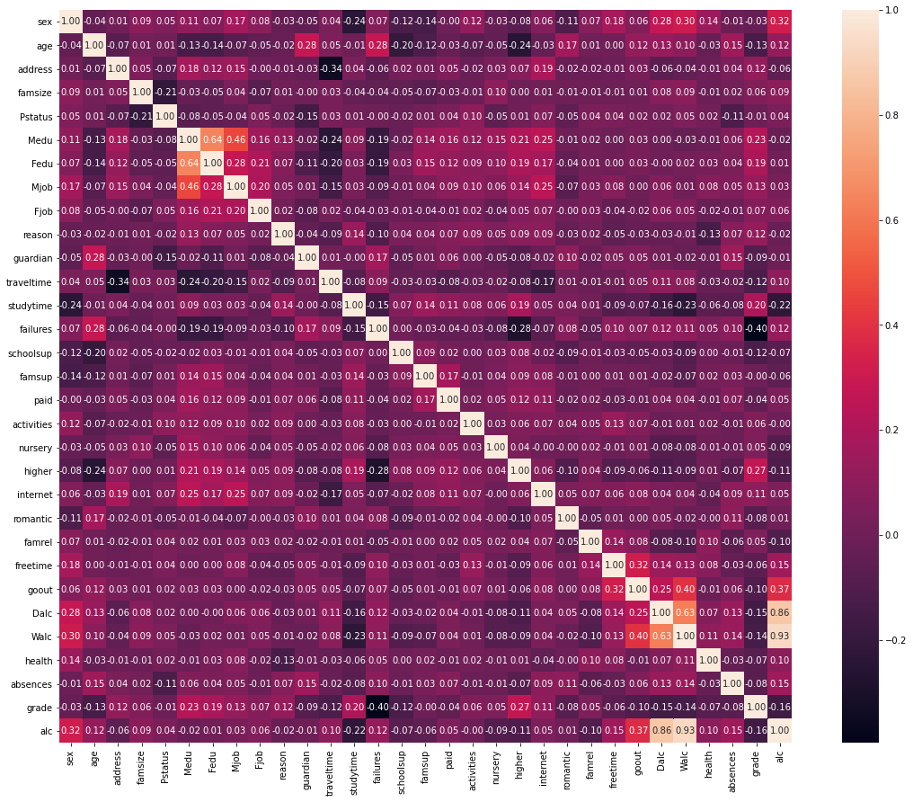
Just from the correlation heatmap, we can have an overview of the impact of alcohol consumption on students. Based on the linear correlation between the target and the features, there is a tendency for students consuming alcohol frequently to have more chance to:
have lower grades
have more absences
hang out more often
not aim to achieve higher education
study less
Among all theses cases, the attributes that are the most correlated with the target are the grades, the study time and if the student is a men.
Impact of alcohol consumption on students life
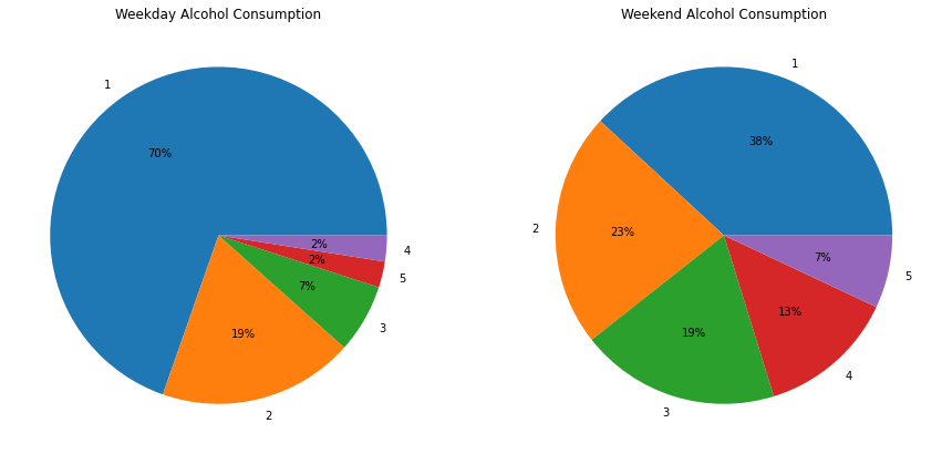
def plot_pie(data, column, ax):"""Plots a pie diagram Args: data: A pandas data frame for the data. columns: A list containing the columns we are interested in. ax: The plt ax from which to plot the pie. """ counts = data[column].value_counts() percent = counts / counts.sum() *100 labels = counts.index ax.pie(x=percent, labels=labels, autopct='%1.0f%%')
The alcohol consumption during workdays is relatively low compared to the weekend consumption. Most students prefer to stay sober during workdays. Let’s see how those behaviors have an impact on students success and life.
<matplotlib.axes._subplots.AxesSubplot at 0x1b1a8863cc8>
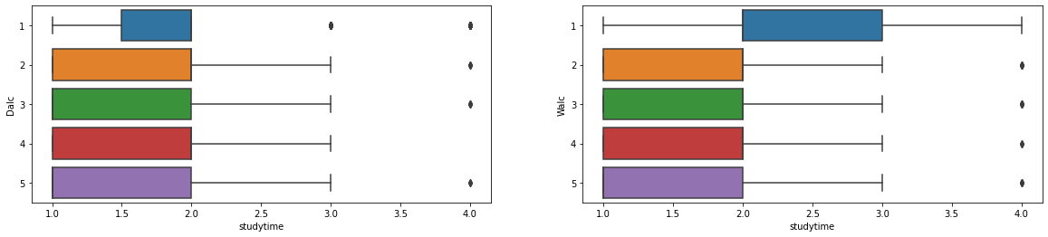
Students who do not drink alcohol during weekdays usually study more than those who do. But the amount of study hours of students who do not drink during weekend is much more than the ones who do.
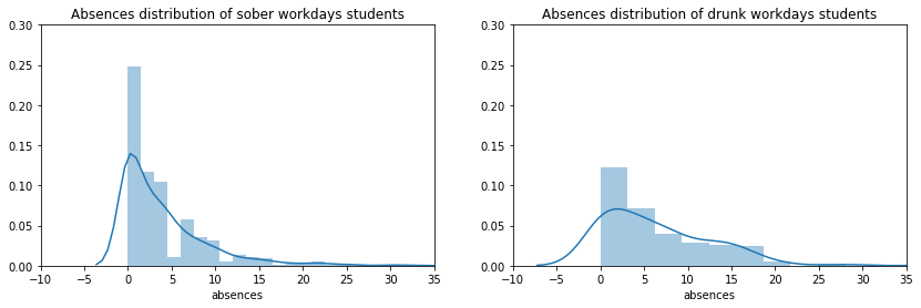
sober_absences = students.loc[students['Dalc'] <=2, 'absences']drunk_absences = students.loc[students['Dalc'] >2, 'absences']_, (ax1, ax2) = plt.subplots(1, 2, figsize=(14, 4))ax1.set_xlim(-10, 35)ax2.set_xlim(-10, 35)ax1.set_ylim(0, 0.30)ax2.set_ylim(0, 0.30)ax1.set_title('Absences distribution of sober workdays students')ax2.set_title('Absences distribution of drunk workdays students')sns.distplot(sober_absences, ax=ax1)sns.distplot(drunk_absences, ax=ax2)
<matplotlib.axes._subplots.AxesSubplot at 0x1b1a8de7b08>
Students who drink two times or more a week have a tendency to be more absent in class.
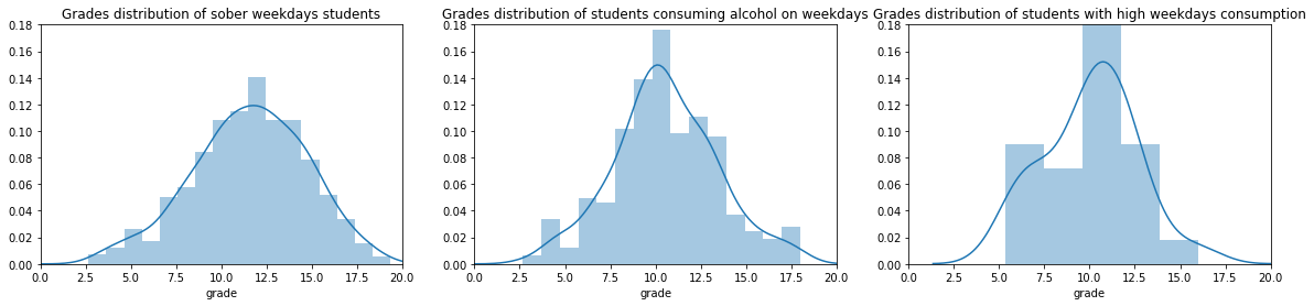
_, (ax1, ax2, ax3) = plt.subplots(1, 3, figsize=(20, 4))sober_grades = students.loc[students['Dalc'] ==1, 'grade']drunk_grades = students.loc[students['Dalc'] >1, 'grade']severe_drunk_grades = students.loc[students['Dalc'] ==5, 'grade']ax1.set_ylim(0, 0.18)ax2.set_ylim(0, 0.18)ax3.set_ylim(0, 0.18)ax1.set_xlim(0, 20)ax2.set_xlim(0, 20)ax3.set_xlim(0, 20)ax1.set_title('Grades distribution of sober weekdays students')ax2.set_title('Grades distribution of students consuming alcohol on weekdays')ax3.set_title('Grades distribution of students with high weekdays consumption')sns.distplot(sober_grades, ax=ax1)sns.distplot(drunk_grades, ax=ax2)sns.distplot(severe_drunk_grades, ax=ax3)
<matplotlib.axes._subplots.AxesSubplot at 0x1b1a7d7e7c8>
Students who drink even a little during workdays have lower grades than those who do not. The impact on grades is much more important for students with severe consumption.
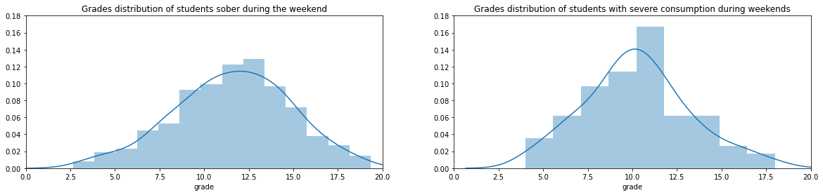
_, (ax1, ax2) = plt.subplots(1, 2, figsize=(20, 4))sober_grades = students.loc[students['Walc'] ==1, 'grade']severe_drunk_grades = students.loc[students['Walc'] ==5, 'grade']ax1.set_ylim(0, 0.18)ax2.set_ylim(0, 0.18)ax1.set_xlim(0, 20)ax2.set_xlim(0, 20)ax1.set_title('Grades distribution of students sober during the weekend')ax2.set_title('Grades distribution of students with severe consumption during weekends')sns.distplot(sober_grades, ax=ax1)sns.distplot(severe_drunk_grades, ax=ax2)
<matplotlib.axes._subplots.AxesSubplot at 0x1b1a8e2e188>
However, even heavy alcohol consumption during the weekend has little impact on student grades. Great news ! We can party during the weekend and it does not affect our productivity.
Pre-processing
In this sections, we will convert the alcohol consumption data to categorical labels The original label goes from 1 to 5 from no consumption to severe consumption. It makes more sense to try to predict the weekly consumption of students so we combined the two attributes by summing them.
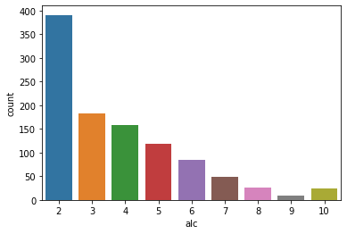
The fourth values seems like a good threshold to create three categorical classes:
\([2, 3]\) little alcohol consumption
\([4, 5]\) moderate alcohol consumption
\([6, 10]\) severe alcohol consumption
sns.countplot(students['alc'])
<matplotlib.axes._subplots.AxesSubplot at 0x1b1a7f9ae88>
# Converting weekly consumption to classesstudents.loc[students['alc'] <=3, 'alc'] =0# little students.loc[(students['alc'] >3) & (students['alc'] <=5), 'alc'] =1# moderatestudents.loc[students['alc'] >5, 'alc'] =2# severe# We need to distinguish categorical from numeric values to fit different distributions# when we will fit the modelnumeric_cols = ['age','traveltime','studytime','failures','famrel','freetime','goout','health','absences','grade','alc']students = students.drop(columns=['Walc', 'Dalc'])is_categorical = []for col in students.columns:if col in numeric_cols: is_categorical.append(0)else: is_categorical.append(1)# Convert data to torch tensorX = torch.from_numpy(students.iloc[:, :-1].values).float()y = torch.from_numpy(students.iloc[:, -1].values).float()
Naive Bayes Classifier
Considering a vector of discrete values \(\boldsymbol{x} \in \{1, \dots, K\}^D\), where \(K\) is the number of values for each feature and \(D\) the number of features. The naive bayes classifier assumes that the data is conditionally independant given the class label i.e \(p(\boldsymbol{x}|y=c)\). This assumption allows us to write the class conditional density as a product: \[\begin{align}
p(\boldsymbol{x} | y = c, \boldsymbol{\theta}) = \prod_{i=1}^{K}p(x_i | y = c, \boldsymbol{\theta}_{ic})
\end{align}\] The model is called “naive” since we do not expect the features to be independent, even conditional on the class label.
Assuming the bayes theorem: \[\begin{align}
P(A|B) = \frac{P(A)P(B|A)}{P(B)}
\end{align}\] To have an easier understanding of the relation between the training of a model and the bayes theorem, let’s reformulate this equation in terms of class and sample: \[\begin{align}
&P(\text{class}|\text{sample}) = \\
&\frac{P(\text{class})P(\text{sample}|\text{class})}{P(\text{sample})}
\end{align}\]
When predicting, we utilize the following approximation: \[\begin{align}
&P(c_j|\boldsymbol{x}) \sim \\
&P(c_j)P(x_i|c_j)\dots P(x_D|c_j)
\end{align}\]
In other words, for each potential class, we multiply the probability of the class (prior) with the probability of finding each features of \(x_i\) in each class \(c_j\) (posterior).
For categorical or binay features, we group the training samples according to each class The form of the class-conditional density depends on the type of each feature. We give some possibilities below:
For real values, we can use the Gaussian distribution: \[\begin{align}
p(\boldsymbol{x} | y = c, \boldsymbol{\theta}) = \prod_{i=1}^{D} \mathcal{N}(x_i| \mu_{ic}, \sigma_{ic}^2)
\end{align}\]
For binary values, we can use a Bernouilli distribution, where \(\mu_{ic}\) is the probability that feature \(i\) occurs in class \(c\): \[\begin{align}
p(\boldsymbol{x} | y = c, \boldsymbol{\theta}) = \prod_{i=1}^{D} \text{Ber}(x_i | \mu_{ic})
\end{align}\]
For categorical features, we can use a Multinouilli distribution, where \(\boldsymbol{\mu}_{ic}\) is an histogram over the possible values for \(x_i\) in class \(c\): \[\begin{align}
p(\boldsymbol{x} | y = c, \boldsymbol{\theta}) = \prod_{i=1}^{D}\text{Cat}(x_i | \boldsymbol{\mu}_{ic})
\end{align}\]
These are the training steps:
group data according to the class label \(c_i\)
compute the prior probability i.e \(p(c_i)\) the proportion of samples inside each class \(c_i\) of the whole training set
for each feature:
if the feature is categorical, compute \(p(\boldsymbol{x_j} | c_i)\) for \(j = 1, \dots, D\) and \(i = 1, \dots, C\):
for each possible values of this feature in the training samples of class \(c_i\), compute the probability that this feature appears in class \(c_i\)
if the feature is continuous, compute \(p(\boldsymbol{x_j} | c_i)\) for \(j = 1, \dots, D\) and \(i = 1, \dots, C\):
compute the mean \(\mu\) and standard deviation \(\sigma\) of the training samples of class \(c_i\) and fit a normal distribution \(\mathcal{N}(\mu, \sigma^2)\)
To predict on a new samples:
for each class \(c_i\), compute \(p(c_i | x)\) as:
multiply the prior of each class \(p(c_i)\) by:
for each features \(k\):
if categorical, multiply by the probabilities calculated earlier \(p(\boldsymbol{x_k} | c_i)\) where \(x_k\) is the value of the input on feature \(k\).
if continuous, multiply by \(\mathcal{N}(x_k | \mu, \sigma^2)\) the likelihood of the gaussian distribution given the input \(x_k\)
return the highest probability \(p(c_i | x)\) of all classes
class NaiveBayesClassifier(BaseEstimator):"""Class for the naive bayes classifier Inherits from sklearn BaseEstimator class to use cross validation. Attributes: offset: An integer to increment the conditional probabilities in order to smooth probabilities to avoid that a posterior probability be 0. is_categorical: A list containing 0 and 1 for indicating if a feature is categorical or numerical. nb_features: An integer for the numbers of feature of the data. nb_class: An integer for the number of classes in the labels. class_probs: A torch tensor for the proportion of each class. cond_probs: A torch tensor for the conditional probability of having a given value on a certain feature in the population of each class. """def__init__(self, offset=1):"""Init function for the naive bayes class"""self.offset = offsetdef fit(self, X, y, **kwargs):"""Fits the model given data and labels as input Args: X: A torch tensor for the data. y: A torch tensor for the labels. """# It is mandatory to pass a list describing if each feature is categorical or numericalif'is_categorical'notin kwargs:raiseValueError('must pass \'is_categorical\' to fit through **kwargs')self.is_categorical = kwargs['is_categorical'] size = X.shape[0]self.nb_features = X.shape[1] y_uvals = y.unique()self.nb_class =len(y_uvals)# Probability of each class in the training setself.class_probs = y.int().bincount().float() / size features_maxvals = torch.zeros((self.nb_features,), dtype=torch.int32)for j inrange(self.nb_features): features_maxvals[j] = X[:, j].max()# All the posterior probabilites cond_probs = [] for i inrange(self.nb_class): cond_probs.append([])# Group samples by class idx = torch.where(y == y_uvals[i])[0] elts = X[idx] size_class = elts.shape[0]for j inrange(self.nb_features): cond_probs[i].append([])ifself.is_categorical[j]:# If categorical# For each featuresfor k inrange(features_maxvals[j] +1):# Count the number of occurence of each value in this feature given the group class# Divided by the number of samples in the class p_x_k = (torch.where(elts[:, j] == k)[0].shape[0] +self.offset) / size_class# Append to posteriors probabilities cond_probs[i][j].append(p_x_k)else:# If numerical features_class = elts[:, j]# Compute mean and std mean = features_class.mean() std = (features_class - mean).pow(2).mean().sqrt()# Store these value to use them for the gaussian likelihood cond_probs[i][j] = [mean, std]self.cond_probs = cond_probsreturn0def gaussian_likelihood(self, X, mean, std):"""Computes the gaussian likelihood Args: X: A torch tensor for the data. mean: A float for the mean of the gaussian. std: A flot for the standard deviation of the gaussian. """return (1/ (2* math.pi * std.pow(2))) * torch.exp(-0.5* ((X - mean) / std).pow(2))def predict(self, X):"""Predicts labels given an input Args: X: A torch tensor containing a batch of data. """iflen(X.shape) ==1: X = X.unsqueeze(0) nb_samples = X.shape[0] pred_probs = torch.zeros((nb_samples, self.nb_class), dtype=torch.float32)for k inrange(nb_samples): elt = X[k]for i inrange(self.nb_class):# Set probability by the prior (class probability) pred_probs[k][i] =self.class_probs[i] prob_feature_per_class =self.cond_probs[i]for j inrange(self.nb_features):ifself.is_categorical[j]:# If categorical get the probability of drawing the value of the input on feature j# inside class i pred_probs[k][i] *= prob_feature_per_class[j][elt[j].int()]else:# If numerical, multiply by the gaussian likelihood with parameters# mean and std of the class i on feature j mean, std = prob_feature_per_class[j] pred_probs[k][i] *=self.gaussian_likelihood(elt[j], mean, std)# Return the highest probability among all classesreturn pred_probs.argmax(dim=1)
Even if the naive bayes model makes a strong assumption that the features are conditionaly independant given the class label, it achieved almost 57% accuracy on three output classes. This model does not perform as well as the more sophisticated models but it is very fast and suited as a baseline model for most classification tasks.
On the other hand, naive bayes models can be descent predictors but they are considered as bad estimators i.e the output probabilities are not to be taken seriously. The naive bayes technique is performing better than logistic regression on small datasets, whereas it is the opposite for large datasets.
Now you can read the next article of this series on Clustering Methods !
Stay in touch
I hope you enjoyed this article as much as I enjoyed writing it!
Feel free to DM me any feedback on LinkedIn or email me directly. It will be highly appreciated.
That's what keeps me going!
Subscribe to get the latest articles from my blog delivered straight to your inbox!
About the author
Axel Mendoza
Senior MLOps Engineer
I'm a Senior MLOps Engineer with 6+ years of experience building production-ML systems.
I write long-form articles on MLOps to help you build too!