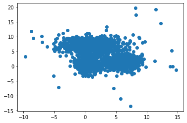
During this experiment, we will implement the K-means clustering and Gaussian Mixture Model algorithms from scratch using Pytorch. The data used for training the unsupervised models was generated to show the distinction between K-means and Gaussian Mixture.
Before starting, feel free to read the previous article of this series.
import osimport mathimport torchimport numpy as npimport pandas as pdimport matplotlib.pyplot as pltfrom sklearn.preprocessing import LabelEncoderfrom sklearn.preprocessing import StandardScaler
def data_generator(cluster_nums, cluster_means, cluster_var, background_range, background_noise_nums):"""Generates data using a mutivariate normal distribution Args: cluster_nums: A positive integer for number of clusters. cluster_means: A list or numpy array describing the mean of each cluster. cluster_var: A list or numpy array describing the variance of each cluster. background_range: A tuple containing two float for the range of the background noise. background_noise_nums: Number of background noise points. Returns: A 2d numpy array. """ data = []for num, mu, var inzip(cluster_nums, cluster_means, cluster_var): data += [np.random.multivariate_normal(mu, np.diag(var), num)] data = np.vstack(data) noise = np.random.uniform(background_range[0], background_range[1], size=(background_noise_nums, data.shape[-1])) data = np.append(data, noise, axis=0)return data
Our goal is to separate the data into groups where the samples in each group are similar.
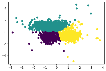
The K-means method is a distance based clustering approach. It is mandatory to standardize the data to prevent the features with higher values to contribute more than the others.
X = StandardScaler().fit_transform(X)X = torch.from_numpy(X).float()
K-Means Clustering
K-means algorithm is an iterative approach that tries to partition a dataset into \(K\) predefined clusters where each data point belongs to only one cluster.
This algorithm works that way:
specify number of clusters \(K\)
randomly initialize one centroid in space for each cluster
for each point, compute the euclidean distance between the point and each centroid and assign the point to the closest centroid
change the centroids values based on the points present in each cluster and repeat the previous step until the centroids do not change anymore
The approach, K-means follows to solve this problem is called Expectation-Maximization. The E-step assign each point to a cluster, and the M-step refines the values of the centroid based on the points inside each cluster.
More formally, the objective function to minimize is as follows: \[\begin{align}
J = \sum_{i=1}^{m} \sum_{k=1}^{K} \mathbb{I}(z_i = k)||x_i - \mu_k||_2^2
\end{align}\] where \(z_i\) is the cluster assigned to \(x_i\) and \(\mu_k\) is the mean of the cluster \(k\).
The E-step is defined as: \[\begin{align}
z_i^{*} = \text{argmin}_{k} ||x_i - \mu_k||_2^2
\end{align}\]
And the M-step is defined as: \[\begin{align}
\mu_k = \frac{1}{\sum_{i=1}^m \mathbb{I}(z_i = k)} \sum_{i=1}^m x_i\mathbb{I}(z_i = k)
\end{align}\]
In practice, we should run multiple K-means with different initialization of the centroids and keep the parameters that minimizes the objective function. Since K-means is a distance based algorithm, is it mandatory to standardize the data.
class KMeansClustering():"""K-Means class implemented in Pytorch Attributes: n_clusters: A integer describing in how many clusters to separate the data. centroids: A torch tensor containing in each column the mean of the n'th cluster. Usage: kms = KMeansClustering(n_clusters=3) pred = kms.fit_transform(X) """def__init__(self, n_clusters=5):"""Inits KmeansClustering class setting the number of clusters"""self.n_clusters = n_clustersself.centroids =Nonedef fit_transform(self, X, n_iter=20):"""Trains the KMeans and clusterize the input data Args: X: A torch tensor for the data to clusterize. n_iters: A integer describing the number of iterations of expectation maximization to perform. """ size = X.shape[0]# Find min and max values to generate a random centroid in this range xmax = X.max(dim=0)[0].unsqueeze(1) xmin = X.min(dim=0)[0].unsqueeze(1) dists = torch.zeros((size, self.n_clusters)) best_loss =1e10 pred =Nonefor _ inrange(n_iter): centroids = (xmin - xmax) * torch.rand((X.shape[1], self.n_clusters)) + xmax old_loss =-1while1:for i inrange(self.n_clusters): # E-step: assign each point to a cluster ctr = centroids[:, i].unsqueeze(1) dists[:, i] = (X - ctr.T).pow(2).sum(dim=1).sqrt() dists_min, labels = dists.min(dim=1)for i inrange(self.n_clusters): # M-step: re-compute the centroids idx = torch.where(labels == i)[0]iflen(idx) ==0:continue centroids[:, i] = X[idx].mean(dim=0) new_loss = dists_min.sum() # Loss: sum distance between points and centroidif old_loss == new_loss:break old_loss = new_lossif new_loss < best_loss: best_loss = new_loss pred = labelsreturn pred
<matplotlib.collections.PathCollection at 0x22813c02548>
The result is pretty satisfying. Each cluster is well separated from each other. Let’s see if we can get a better result using a Gaussian Mixture model.
Gaussian Mixture Model
In order to understand how we train a Gaussian Mixture model, we must explain the expectation-maximization algorithm (EM) first. The EM algorithm is a general technique for finding maximum likelihood solutions for probabilistic models having latent variables. EM is an iterative algorithm that starts from an initial estimate of the parameters of a probabilistic model \(\boldsymbol{\theta}\) and then proceeds to iteratively update \(\boldsymbol{\theta}\) until convergence. This algorithm consists to iteratively apply an expectation step and a maximization step.
Let’s consider the EM algorithm for a multivariate Gaussian Mixture model with \(K\) mixture components, observed variables \(\boldsymbol{X}\) and latent variables \(\boldsymbol{Z}\) such as:
\[\begin{aligned}
P(\boldsymbol{x}_i | \boldsymbol{\theta}) &= \sum_{k=1}^{K} \pi_k P(\boldsymbol{x}_i | \boldsymbol{z}_i, \boldsymbol{\theta}_k)\\
&= \sum_{k=1}^{K} P(\boldsymbol{z}_i = k) \mathcal{N}(\boldsymbol{x}_i; \boldsymbol{\mu}_k, \boldsymbol{\Sigma}_k)
\end{aligned}\]
where each component of the mixture model is the normal distribution. Let’s see why the MLE of a gaussian mixture model is hard to compute. The likelihood of a gaussian mixture distribution is: \[\begin{align}
&L(\boldsymbol{\theta} | \boldsymbol{X}) = \\
&\prod_{i=1}^N\sum_{k=1}^{K} \pi_k \mathcal{N}(\boldsymbol{x}_i; \boldsymbol{\mu}_k, \boldsymbol{\Sigma}_k)
\end{align}\]
This the log-likelihood is as follows: \[\begin{align}
&\mathcal{L}(\boldsymbol{\theta} | \boldsymbol{X}) = \\
&\sum_{i=1}^N \log\left(\sum_{k=1}^{K} \pi_k \mathcal{N}(\boldsymbol{x}_i; \boldsymbol{\mu}_k, \boldsymbol{\Sigma}_k)\right)
\end{align}\]
Because of the sum inside the \(\log\), we cannot estimate \(\boldsymbol{\mu}_k\) and \(\boldsymbol{\sigma^2}\) without knowing \(\boldsymbol{Z}\). That is why we would use EM in this kind of situation.
The EM algorithm has two steps, the expectation step known as E-step, assigns to each data point the probability that they belong to each components of the mixture model. Whereas the maximization step, known as M-step, re-evaluate the parameters of each mixture component based on the estimated values generated in the E-step.
More formally, during the E-step, we calculate the likelihood of each data point using the estimated parameters: \[\begin{align}
&K = \frac{1}{\sqrt{(2\pi)^m|\boldsymbol{\Sigma}_k|}} \\
&f(\boldsymbol{x_i}|\mu_k, \boldsymbol{\Sigma}_k) = \\
&K\exp\left(-\frac{(\boldsymbol{x}_i - \boldsymbol{\mu}_k)^\top \boldsymbol{\Sigma}_k^{-1}(\boldsymbol{x}_i - \boldsymbol{\mu}_k)}{2}\right)
\end{align}\] where \(m\) is the number of features in the input data.
Then we compute the probability that \(\boldsymbol{x}_i\) came from the \(k^{th}\) gaussian distribution: \[\begin{align}
p_{ik} = \frac{\pi_k f(\boldsymbol{x_i}|\mu_k, \boldsymbol{\Sigma}_k)}{\sum_{j=1}^{K} \pi_j f(\boldsymbol{x_i}|\mu_j, \boldsymbol{\Sigma}_j)}
\end{align}\]
For the M-step, we update the parameters of the mixture as follows:
\[\begin{aligned}
\pi_k &= \frac{1}{N}\sum_{i=1}^{N} p_{ik}\\
\boldsymbol{\mu}_k &= \frac{1}{\sum_{i=1}^{N} p_{ik}} \sum_{i=1}^{N} p_{ik} \boldsymbol{x_i}\\
\boldsymbol{\Sigma}_k &= \frac{1}{\sum_{i=1}^{N} p_{ik}} \sum_{i=1}^{N} p_{ik} (\boldsymbol{x}_i - \boldsymbol{\mu}_k) (\boldsymbol{x}_i - \boldsymbol{\mu}_k)^\top
\end{aligned}\]
class GaussianMixture():"""Gaussian Mixture model class separating data in clusters The KMeans class is used to initialize the probabilities p_ik of each sample. Attributes: n_components: An integer for the number of gaussian distributions in the mixture. n_iter: A positive integer for the number of iterations to perform e-steps and m-steps. priors: A torch tensor containing the probabilities of each class. mu: A torch tensor for the mean of each gaussian. sigma: A torch tensor for the covariance of each gaussian. likelihoods: A torch tensor containing the likelihoods of each data in regards to each gaussian. probs: A torch tensor holding the probabilities for each data to belong to each gaussian. Usage: gmm = GaussianMixture(n_components=3, n_iter=3) pred = gmm.fit_predict(X) """def__init__(self, n_components, n_iter):"""Inits the GaussianMixture class by setting n_components and n_iter"""self.n_components = n_componentsself.n_iter = n_iterdef gaussian_likelihood(self, X, n):"""Returns the gaussian likelihood of X from the nth gaussian""" two_pi = torch.tensor(2* math.pi, dtype=torch.float64) fact =1/ torch.sqrt(torch.pow(two_pi, X.shape[0]) * torch.det(self.sigma[n])) X_minus_mu = X -self.mu[n].T sigma_inv = torch.inverse(self.sigma[n])return fact * torch.exp(-0.5* X_minus_mu.mm(sigma_inv).mm(X_minus_mu.T))def e_step(self, X):"""Assigns to each data the probability to belong to each gaussian"""for j inrange(self.n_components):for i inrange(self.n_samples):self.likelihoods[i, j] =self.gaussian_likelihood(X[i], j)# Tensor to hold the probabilities that each data belongs to each gaussian prob_num =self.priors.T *self.likelihoods prob_den = prob_num.sum(dim=1).unsqueeze(1)self.probs = prob_num / prob_dendef m_step(self, X):"""Re-computes the parameters of each gaussian component"""for j inrange(self.n_components): probs_j =self.probs[:, j] # All probabilities from the j'th guassian probs_j_sum = probs_j.sum()self.priors[j] = probs_j.sum() /self.n_samples probs_j_uns = probs_j.unsqueeze(1)# Recomputes the means of each gaussian based on the probabilities of# each data.self.mu[j] = (probs_j_uns * X).sum(dim=0).unsqueeze(1)self.mu[j] /= probs_j_sum# Recomputes the covariance matrix of each data X_minus_mu = X -self.mu[j].Tself.sigma[j].fill_(0.)for i inrange(self.n_samples): row = X_minus_mu[i, :].unsqueeze(1)self.sigma[j] += probs_j[i] * row.mm(row.T)self.sigma[j] /= probs_j_sumdef fit_predict(self, X):"""Trains the models and returns the clusters"""self.n_samples = X.shape[0]self.n_features = X.shape[1]self.sigma = torch.zeros((self.n_components, self.n_features, self.n_features), dtype=torch.float64)self.mu = torch.zeros((self.n_components, self.n_features, 1), dtype=torch.float64)self.priors = torch.zeros((self.n_components, 1), dtype=torch.float64).fill_(1/self.n_components)# Initialize the probabilities of each samples to belong# to each gaussian by a KMeans kms = KMeansClustering(n_clusters=self.n_components) pred = kms.fit_transform(X).unsqueeze(1)self.probs = torch.zeros(self.n_samples, self.n_components)self.probs.scatter_(1, pred, 1)# Set the covariance parameter of each components to the# covariance of the data X_m = X - X.mean() X_cov = X_m.T.mm(X_m)for j inrange(self.n_components):self.sigma[j] = X_cov.clone()# Select a random sample as the mean of each gaussianself.mu[j] = X[torch.randint(0, self.n_samples, (1,))].Tself.likelihoods = torch.zeros((self.n_samples, self.n_components), dtype=torch.float64)self.m_step(X) # Start with m_step to compute params of gaussians based on KMeans probabilitiesfor _ inrange(self.n_iter):self.e_step(X)self.m_step(X)returnself.probs.argmax(dim=1)
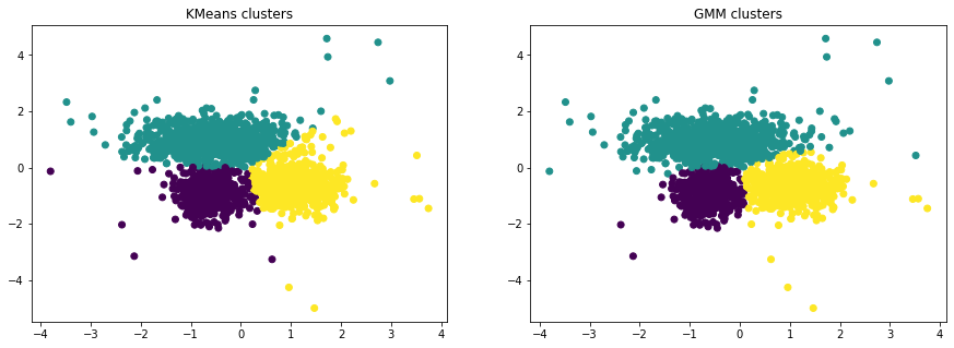
The KMeans algorithm can only describe spherical clusters while GMM can express elliptic clusters. In this experiment, the GMM undoubtably found the gaussian distributions that we generated. Whereas KMeans did a great job to separate the data but still lacks expressivity for clustering elliptic clusters.
KMeans is significantly faster and simpler than other EM algorithm, but for data that has different sized and shaped clusters, GMM does a better job. However, GMM is known to be unstable. Indeed, the clusters can be a little bit different each time.
If we had to choose one assertion to take out from this experiment, it would be that clustering methods are very powerful techniques suited for finding latent or missing variables.
Want to keep learning ? Jump right in the next article.
Stay in touch
I hope you enjoyed this article as much as I enjoyed writing it!
Feel free to DM me any feedback on LinkedIn or email me directly. It will be highly appreciated.
That's what keeps me going!
Subscribe to get the latest articles from my blog delivered straight to your inbox!
About the author
Axel Mendoza
Senior MLOps Engineer
I'm a Senior MLOps Engineer with 6+ years of experience building production-ML systems.
I write long-form articles on MLOps to help you build too!