During this experiment, we will train logistic regression on diabetes data, from scratch using Pytorch. Before starting, feel free to explore the previous article of this series: .
The Pima Indians Diabetes Database has been gathered by the National Institute of Diabetes and Digestive and Kidney Diseases. The objective of this dataset is to diagnostically predict whether or not a patient has diabetes, based on certain diagnostic measurements included in the dataset.
Several constraints were placed on the selection of these instances from a larger database. In particular, all patients here are females at least 21 years old of Pima Indian heritage. This dataset contains the following features:
Pregnancies
Glucose
BloodPressure
SkinThickness
Insuline
BMI
DiabetesPedigreeFunction
Age
Outcome (has diabetes or not)
import osimport torchimport numpy as npimport pandas as pdimport seaborn as snsimport matplotlib.pyplot as pltfrom sklearn.preprocessing import StandardScalerfrom sklearn.metrics import classification_reportfrom sklearn.metrics import confusion_matrixfrom sklearn.model_selection import train_test_split
On this sample of data, the standard devitation of the columns looks reasonably high except for the DiabetesPedigree but it is acceptable because the mean is relatively low. A feature having low std is likely to provide close to no information to the model. Which is not the case here.
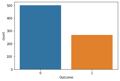
sns.countplot(x='Outcome', data=diabetes)
<matplotlib.axes._subplots.AxesSubplot at 0x14ccf75a2c8>
The target distribution is very unbalanced with two times more negative than positives.
<matplotlib.axes._subplots.AxesSubplot at 0x14ccf67da48>
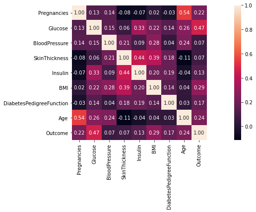
The glucose level, BMI, age and number of pregnancies are highly correlated with the outcome. Suprisingly, the insulin level is not very correlated with the outcome. Most likely because the insulin is correlated with the glucose and the glucose has 0.47 correlation with the target.
<matplotlib.axes._subplots.AxesSubplot at 0x14ccf2508c8>
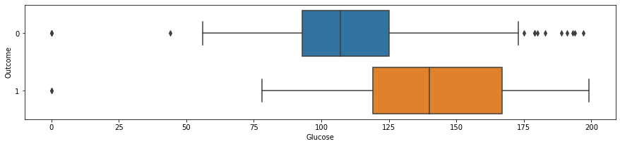
For patient with diabetes, the glucose level is significantly higher. In other words, a patient with high glucose level is very likely to have diabetes.
<matplotlib.axes._subplots.AxesSubplot at 0x14ccdeb66c8>
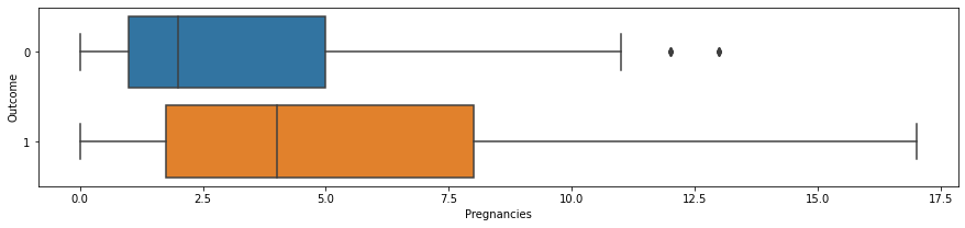
Surprisingly, the number of pregnancies is correlated with diabetes.
Data Preparation
Convert data to Torch tensors
X = diabetes.iloc[:, :-1].valuesy = torch.from_numpy(diabetes.iloc[:, -1].values).float().unsqueeze(1)# Standardize the dataX = StandardScaler().fit_transform(X)X = torch.from_numpy(X).float()# Add column of ones for the biasones_col = torch.ones((X.shape[0], 1), dtype=torch.float32)X = torch.cat([ones_col, X], axis=1)
Create the Training Split
X_train, X_test, y_train, y_test = train_test_split(X, y, random_state=42, test_size=0.25)
Logistic Regression
The prediction of a logistic model is as follow: \[\begin{align}
\hat{y} = \sigma(\boldsymbol{X}\boldsymbol{w})
\end{align}\] Where \(\sigma\) is the sigmoid or logit function: \[\begin{align}
\sigma(\boldsymbol{x}) = \frac{1}{1 + \exp(-x)}
\end{align}\] The prediction \(\hat{y}\) is obtained by matrix multiplication between the input \(\boldsymbol{X}\) and the weights of the model \(\boldsymbol{w}\) given as input to the logit function. The sigmoid function is used here because it squashes the input in the \([0, 1]\) range suitable for describing a Bernouilli distribution.
Where the Bernouilli cases are:
The patient has diabetes with \(p\) probability
The patient does not have diabetes with \(1 - p\) probability
It is important to note that the bias is included in \(\boldsymbol{X}\) as a column of ones.
Training a classification model can be expressed as maximizing the likelihood of the observed data.
In practice, maximizing the likelihood is equivalent to minimize the negative log likelihood: \[\begin{align}
L(\boldsymbol{\theta}) = - \frac{1}{N}\sum_{i=1}^{n}\boldsymbol{y_i}\log(\hat{\boldsymbol{y}}_i)
\end{align}\] Because we dealing with a binary target, it is appropriate to use the binary cross entropy: \[\begin{align}
L(\boldsymbol{\theta}) = &- \frac{1}{N}\sum_{i=1}^{n}\boldsymbol{y_i}\log(\hat{\boldsymbol{y}}_i) \\
&+ (1 - \boldsymbol{y_i})\log(1 - \hat{\boldsymbol{y}}_i)
\end{align}\]
Gradient Descent
We will use Gradient Descent to train the logistic regression model. The Gradient descent method takes steps proportional to the negative of the gradient of a function at a given point, in order to iteratively minimize the objective function.The gradient generalizes the notion of derivative to the case where the derivative is with respect to a vector: the gradient of \(f\) is the vector containing all of the partial derivatives, denoted \(\nabla_{\boldsymbol{x}}f(\boldsymbol{x})\).
The directional derivative in direction \(\boldsymbol{u}\) (a unit vector) is the slope of the function \(f\) in direction \(\boldsymbol{u}\). In other words, the directional derivative is the derivative of the function \(f(\boldsymbol{x} + \sigma \boldsymbol{u})\) with respect to \(\sigma\) close to 0. To minimize \(f\), we would like to find the direction in which \(f\) decreases the fastest. We can do this using the directional derivative: \[\begin{align}
&\min_{\boldsymbol{u}, \boldsymbol{u}^\top \boldsymbol{u} = 1}{\boldsymbol{u}^\top \nabla_{\boldsymbol{x}} f(\boldsymbol{x})} \\
&= \min_{\boldsymbol{u}, \boldsymbol{u}^\top \boldsymbol{u} = 1}{||\boldsymbol{u}||_2 ||\nabla_{\boldsymbol{x}}f(\boldsymbol{x})||_2 \cos \theta}
\end{align}\] ignoring factors that do not depend on \(\boldsymbol{u}\), this simplifies to \(\min_{u}{\cos \theta}\). This is minimized when \(\boldsymbol{u}\) points in the opposite direction as the gradient. Each step of the gradient descent method proposes a new point: \[\begin{align}
\boldsymbol{x'} = \boldsymbol{x} - \epsilon \nabla_{\boldsymbol{x}}f(\boldsymbol{x})
\end{align}\] where \(\epsilon\) is the learning rate. In the context of logistic regression, the gradient descent is as follow: \[\begin{align}
\boldsymbol{w} = \boldsymbol{w} - \epsilon \nabla_{\boldsymbol{w}}L(\boldsymbol{\theta})
\end{align}\] where: \[\begin{align}
\nabla_{\boldsymbol{w}}L(\boldsymbol{\theta}) = \frac{1}{N}\boldsymbol{X}^\top(\sigma(\boldsymbol{X}\boldsymbol{w}) - \boldsymbol{y})
\end{align}\] Here is a nice explanation of how to find the gradient of the binary cross entropy throug this link.
Training the Model
def sigmoid(x):"""Sigmoid function that squashes the input between 0 and 1"""return1/ (1+ torch.exp(-x))def predict(X, weights):"""Pedicts the class given the data and the weights Args: X: A torch tensor for the input data. weights: A torch tensor for the parameters calculated during the training of the Logistic regression. """return sigmoid(X.mm(weights))
def binary_cross_entropy(y_true, y_pred):"""Loss function for the training of the logistic regression We add an epsilon inside the log functions to avoid Nans. Args: y_true: A torch tensor for the labels of the data. y_pred: A torch tensor for the values predicted by the model. """ fact =1/ y_true.shape[0]return-fact * (y_true * torch.log(y_pred +1e-10) + (1- y_true) * torch.log(1- y_pred +1e-10 )).sum()
def train_logit_reg(X, y_true, weights, lr=0.001, it=2000):"""Trains the logistic regression model Args: X: A torch tensor for the training data. y: A torch tensor for the labels of the data. weights: A torch tensor for the learning parameters of the model. lr: A scalar describing the learning rate for the gradient descent. it: A scalar for the number of steps in the gradient descent. """for _ inrange(it): y_pred = predict(X, weights) err = (y_pred - y_true) grad = X.T.mm(err) weights -= lr * grad bn_train = binary_cross_entropy(y_true, y_pred).item()return weights, bn_train
# Training the modelweights = torch.ones((X.shape[1], 1), dtype=torch.float32)weights, bn_train = train_logit_reg(X_train, y_train, weights)y_pred = predict(X_test, weights)print('Binary cross-entropy on the train set:', bn_train)
Binary cross-entropy on the train set: 0.4595394730567932
Testing the model
# Test the modelbn_test = binary_cross_entropy(y_test, y_pred).item()print('Binary cross-entropy on the test set:', bn_test)
Binary cross-entropy on the test set: 0.5321948528289795
Accuracy on test set
To compute the accuracy, we have to find the best threshold to convert our probability output in binary values.
def get_binary_pred(y_true, y_pred):"""Finds the best threshold based on the prediction and the labels Args: y_true: A torch tensor for the labels of the data. y_pred: A torch tensor for the values predicted by the model. """ y_pred_thr = y_pred.clone() accs = [] thrs = []for thr in np.arange(0, 1, 0.01): y_pred_thr[y_pred >= thr] =1 y_pred_thr[y_pred < thr] =0 cur_acc = classification_report(y_test, y_pred_thr, output_dict=True)['accuracy'] accs.append(cur_acc) thrs.append(thr) accs = torch.FloatTensor(accs) thrs = torch.FloatTensor(thrs) idx = accs.argmax() best_thr = thrs[idx].item() best_acc = accs[idx].item() y_pred[y_pred >= best_thr] =1 y_pred[y_pred < best_thr] =0return y_pred
With a threshold of 0.66, we achieve an accuracy of 78% which is quite good for a linear model.
Polynomial Logistic Regression
In this section, we will add some polynomial features to the logistic regressor. It is the same principle as the logistic regression except that \(\boldsymbol{X}\) is the concatenation of \(\boldsymbol{X_1} \dots \boldsymbol{X_m}\) where \(m\) is the degree of the polynomial function and \(\boldsymbol{w}\) is the concatenation of \(\boldsymbol{w_1} \dots \boldsymbol{w_m}\) such as: \[\begin{align}
\boldsymbol{y} = \sigma(\boldsymbol{w}_0 + \boldsymbol{X}\boldsymbol{w}_1 + \dots + \boldsymbol{X}^m\boldsymbol{w}_m)
\end{align}\] This method is still linear because predicting \(\hat{y} = \sigma(\boldsymbol{X}\boldsymbol{w})\) is still linear in the parameters.
X = torch.from_numpy(diabetes.iloc[:, :-1].values).float()y = torch.from_numpy(diabetes.iloc[:, -1].values).float().unsqueeze(1)
def create_poly_features(X, degree=2):"""Creates the augmented features for the polynomial model This function concatenates the augmented data into a single torch tensor. Args: X: A torch tensor for the data. degree: A integer for the degree of the polynomial function that we model. """iflen(X.shape) ==1: X = X.unsqueeze(1) ones_col = torch.ones((X.shape[0], 1))# Standardize the output to avoid exploding gradients X_cat = X.clone() X_cat = (X_cat - X_cat.mean()) / X_cat.std() X_cat = torch.cat([ones_col, X_cat], axis=1)for i inrange(1, degree): X_p = X.pow(i +1) X_p = torch.from_numpy(StandardScaler().fit_transform(X_p)).float() X_cat = torch.cat([X_cat, X_p], axis=1)return X_catdef create_weights(features):"""Creates a column of ones"""return torch.ones((features.shape[1], 1), dtype=torch.float32)
features = create_poly_features(X, degree=2)X_train, X_test, y_train, y_test = train_test_split(features, y, random_state=42, test_size=0.25)weights = create_weights(X_train)weights, bn_train = train_logit_reg(X_train, y_train, weights, it=10000)y_pred = predict(X_test, weights)print('Binary cross-entropy on the train set:', bn_train)
Binary cross-entropy on the train set: 0.44449102878570557
The polynomial logistic regression model overfitted compared to the classic logistic regression model because it lost 1% accuracy on the test set.
For some very highly correlated data, logistic regression without polynomial features has better performance than with polynomial features.
Logistic regression is a very simple and interpretable model suited as a baseline in most classification problems. However, it does not perform well when the feature space is large. In fact, it is difficult to compute feature transformation (such as polynomials) when the data doesn’t fit in ram.
Still interested in improving your machine learning knowledge ? You can read the next article on K-Nearest Neighbors.
Stay in touch
I hope you enjoyed this article as much as I enjoyed writing it!
Feel free to DM me any feedback on LinkedIn or email me directly. It will be highly appreciated.
That's what keeps me going!
Subscribe to get the latest articles from my blog delivered straight to your inbox!
About the author
Axel Mendoza
Senior MLOps Engineer
I'm a Senior MLOps Engineer with 6+ years of experience building production-ML systems.
I write long-form articles on MLOps to help you build too!