During this experiment, we will investigate the maths and implement Decision Trees, Random Forests and Adaboost. We will use Pytorch to create and train these algorithms to predict heart diseases.
Before starting, read the previous article of this series if you haven’t already.
Heart Disease Dataset
The models will be trained using the Heart Disease Dataset. Fourteen features were selected among 76 attributes:
age: age in years
sex:
1: male
0: female
cp: chest pain type
0: asymptomatic
1: atypical angina
2: non-anginal pain
3: typical angina
trestbps: resting blood pressure
chol: serum cholestoral in mg/dl
fbs: fasting blood sugar > 120 mg/dl
restecg: resting electrocardiographic results
0: showing probable or definite left ventricular hypertrophy by Estes’ criteria
1: normal
2: having ST-T wave abnormality (T wave inversions and/or ST elevation or depression of > 0.05 mV)
thalach: maximum heart rate achieved
exang: exercise induced angina
oldpeak: ST depression induced by exercise relative to rest
slope: the slope of the peak exercise ST segment
1: upsloping
2: flat
3: downsloping
ca: number of major vessels (0-3) colored by flourosopy
thal:
3 : fixed defect
6 : normal
7 : reversable defect
disease:
0: artery diameter narrowing < 50%
1-3: artery diameter narrowing > 50%, close to 3 is very severe
import osimport torchimport pandas as pdimport numpy as npimport seaborn as snsimport matplotlib.pyplot as pltfrom pprint import pprintfrom sklearn.model_selection import train_test_splitfrom sklearn.base import BaseEstimatorfrom sklearn.model_selection import cross_val_score
# The data does not include the columns names, we did a little trick to add themcolumns = {'63.0' : 'age','1.0' : 'sex','1.0.1' : 'cp','145.0' : 'trestbps','233.0' : 'chol','1.0.2' : 'fbs','2.0' : 'restecg','150.0' : 'thalach','0.0' : 'exang','2.3' : 'oldpeak','3.0' : 'slope','0.0.1' : 'ca','6.0' : 'thal','0' : 'disease'}hdisease.rename(columns=columns, inplace=True)
Replacing missing values
# Remove the severity of the disease, 0: healthy, 1: sickhdisease.loc[hdisease['disease'] >1, 'disease'] =1# Setting gather unknown value and assign a new class for themhdisease.loc[hdisease['ca'] =='?', 'ca'] =4.0hdisease.loc[hdisease['thal'] =='?', 'thal'] =0.0# Setting all values to floathdisease = hdisease.astype(float)
<matplotlib.axes._subplots.AxesSubplot at 0x20902f1b088>
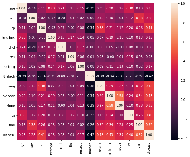
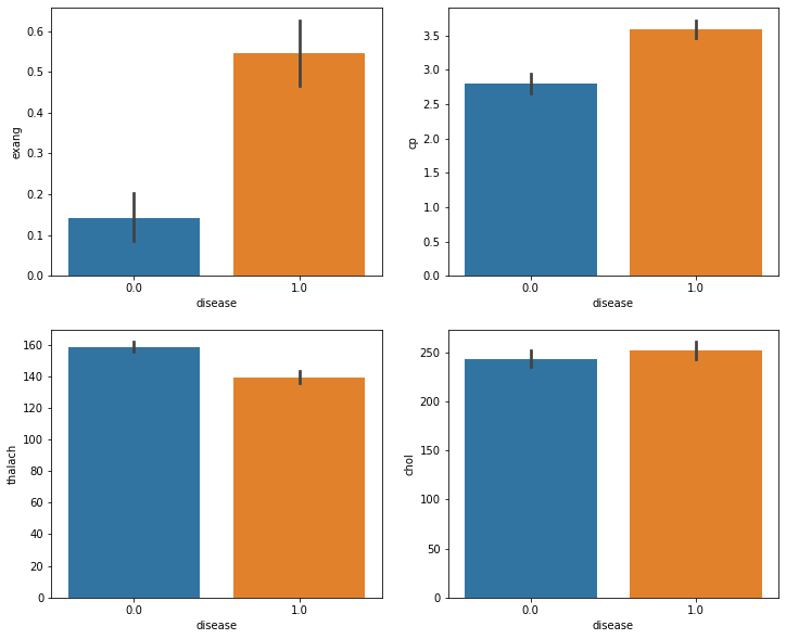
Most features are highly correlated to the disease column. By interpreting the barplots of healthy and sick patients, it is likely that a patient with heart disease will have the following caracteristics:
cp: more chest pain
thalach: a lower maximum heart rate, surprisingly, high beats per minute is a signal of heart health
exang: increase pain when exercising
cholesterol levels are similar through sick and healthy patient: no direct link with heart disease
Decision Trees
Decision trees are defined by recursively partitioning the input space into regions. Each region is partitioned into sub-regions up to a leaf node. Space is sub-divided into non overlapping regions based on some criteria at each node. Once created, a tree can be navigated with a new sample of data following each branch according to the conditions. Each leaf node maps the input to a class or continuous value depending on the task. To understand how to grow a tree, we must introduce the gini index first. Assuming that \(D\) is the data in a leaf and \(N\) the number of samples in \(D\), we estimate the class-conditional probability as follow: \[
\hat{\pi}_c = \frac{1}{N} \sum_{i \in D}\mathbb{I}(y_i = c)
\] where \(c\) are the classes of the target. The Gini index of a given leaf is: \[
G_{l} = \sum_{c=1}^{C}\hat{\pi}_c(1 -\hat{\pi}_c) = 1 - \sum_{c=1}^{C}\hat{\pi}^2_c
\]
To have the Gini index of a split, we compute the Gini index on each of its leaves and multiply each of them by the proportion of samples in each leaves and sum both values:
\[
G_{Node} = \sum_{i=1}^{K} \frac{k_{li}}{U}G_{li}
\] where \(K\) is the number of leaves of the node, \(k_{li}\) is the number of samples in the leaf \(i^{th}\) leaf and \(U\) is the number of sample to split.
In the case of categorical inputs, the most common approach is to consider the split condition as \(x_{ij} = c_k\) or \(x_{ij} \neq c_k\), for each possible class label \(c_k\). The rule to perform a split on a node is as follows:
if the node is in the maximum depth of the tree, keep it as a leaf.
for each attribute, we try all the possible thresholds and compute the Gini index of each split, the threshold across all attributes that minimize the Gini index is selected.
a node is said pure if the split generates a empty leaf, if a node is pure, it is set as a leaf.
if the node has a lowest score than the Gini index of the best split, we keep it as a leaf.
# Check which data are categorical or notis_categorical = []for col in hdisease.columns:# If less than 9 unique values, than the feature is categorical is_categorical.append(int(len(np.unique(hdisease[col])) <9))# Convert to Pytorch tensoris_categorical = torch.tensor(is_categorical)[:-1]
# Convert data to numpydata = hdisease.values# Get unique values of the targetutarget = torch.from_numpy(np.unique(data[:, -1]))
X = torch.from_numpy(data[:, :-1])y = torch.from_numpy(data[:, -1]).int()
class Node():"""Base class for a tree node We will use a single class to have the options to build a Decision Tree, a Random Forest and Adaboost. Attributes: X: A torch tensor for the data. y: A torch tensor for the labels. is_categorical_list: A list of boolean, 1 if the features is categorical, 0 otherwise. max_depth: A positive integer for the depth of the tree. columns: A list of the name of each column. depth: A positive integer for the depth of the node. nb_features: A positive integer for selecting a number of random features for the split. Only used when training a Random Forest. weights: A torch tensor for computing the weighted gini index. Only used when training Adaboost. col_perm: A torch tensor of the permuted column. Only for Random Forests. X_full: A torch tensor that is keeping the whole data in case we shuffle the input for training a Random Forest. col_full: A list that keeps the whole feature names. Only for Random Forests. is_catfull: A list that keeps the whole is_categorical_list if training a Random Forest. size: A positive integer for the number of samples. nb_features: A positive integer for the number of features cutoff: A float for the splitting value of the node. col: A positive integer as an index for which column to apply the condition for the split. left: A Node class for the left child node. right: A Node class for the right child node. """def__init__(self, X, y, is_categorical, max_depth, columns, depth=0, nb_features=0, weights=None):"""Init function of the class This function builds the whole tree, recursively creating each child node down to the leaves. Args: Described in the attribute section of the class """# If training random forest if nb_features !=0:self.col_perm = torch.randperm(X.shape[1])[:nb_features]# We have to keep the permutated data as well as the full data# because we have to pass the full data to the child nodesself.X = X[:, self.col_perm]self.X_full = Xself.columns = columns[self.col_perm]self.col_full = columnsself.is_categorical_list = is_categorical[self.col_perm]self.is_catfull = is_categoricalelse:# Regular training of the decision treeself.X = Xself.columns = columnsself.is_categorical_list = is_categorical# Weights are used to compute a weighted gini index# Only when training AdaBoostself.weights = weightsself.y = yself.size =float(X.shape[0])# Prediction if the node will turn into a leaf, or split valueself.cutoff =None# Column to check for splitting the data self.col =None# Child nodesself.left =Noneself.right =None# Whether or not the split value is categoricalself.depth = depthself.nb_features = nb_features# If the node contains only one label, it is set as a leafifself.is_pure() or depth == max_depth orself.X.shape[0] ==1:# Select the predominant categorical value and set it as the predictionself.make_leaf()return# Computing the gini index on the population before the split gini_n =self.gini(y, self.weights) params =self.find_best_split() gini_s = params[0]# If no improvement, make the node as a leafif gini_s >= gini_n:self.make_leaf()else:self.make_split(params, max_depth)def gini(self, y, weights=None):"""Computes the gini index Args: y: A torch tensor for the labels of the data. weights: If training a Random Forest, the weights associated with each sample. """if weights isNone:# Regular gini index pi = y.bincount() /float(y.shape[0])else:# Weighted gini index pi =self.get_weighted_population(y, weights)return1- pi.pow(2).sum()# For weighted gini index:def get_weighted_population(self, y, weights):"""Computes the weighted gini index Instead of counting the samples for each class we count the weights of each class and divide by the sum of the weights Args: y: A torch tensor for the labels of the data. weights: If training a Random Forest, the weights associated """ pi = torch.zeros((2,), dtype=torch.float32) idx_0 = torch.where(y ==0)[0] idx_1 = torch.where(y ==1)[0] pi[0] = weights[idx_0].sum() pi[1] = weights[idx_1].sum()return pi / weights.sum()def clean_attributes(self):"""Cleans variables that are not usefull to predict"""del(self.X)del(self.y)del(self.weights)del(self.size)ifself.nb_features !=0:del(self.X_full)del(self.col_full)del(self.is_catfull)del(self.colperm)del(self.nb_features)def is_pure(self):"""Checks if the node is pure The node is pure if there is only one label in the population """returnlen(self.y.unique()) ==1def get_label(self):"""Returns the most present label as a prediction if the node turns to a leaf"""ifself.weights isNone:returnself.y.bincount().argmax().item()else:returnself.get_weighted_population(self.y, self.weights).argmax().item()def make_leaf(self):"""Makes the node a leaf"""self.cutoff =self.get_label()self.clean_attributes()def make_split(self, params, max_depth):"""Performs the split Args: params: See find_best_split function max_depht: A positive integer for the maximum of the tree. """self.col = params[1]self.cutoff = params[2]# Save the categorical boolean of the selected column for the predict methodself.var_categorical =self.is_categorical_list[self.col].item()# Recursively split by creating two instances of the Node class using the two groupsifself.nb_features !=0: cols =self.col_full categorical_list =self.is_catfullelse: cols =self.columns categorical_list =self.is_categorical_list# Creating child nodes based on the best params# If training Random Forest, we pass nb_features# If training AdaBoost, we pass the weightsself.left = Node(X=params[3][0], y=params[3][1], is_categorical=categorical_list, max_depth=max_depth, columns=cols, depth=self.depth +1, nb_features=self.nb_features, weights=params[5])self.right = Node(X=params[4][0], y=params[4][1], is_categorical=categorical_list, max_depth=max_depth, columns=cols, depth=self.depth +1, nb_features=self.nb_features, weights=params[6])self.clean_attributes()def gini_split(self, idx_g_1, idx_g_2, cutoff, feature_idx, best_params):"""Computes the gini index of the future split Args: idx_g_1: A torch tensor for the indices of the first group. idx_g_2: A torch tensor for the indices of the second group. cutoff: A float for the split value. feature_idx: A positive integer for the index of the feature to test. best_params: See function find_best_split """ g_1 =self.y[idx_g_1].squeeze(1) g_2 =self.y[idx_g_2].squeeze(1)ifself.weights isNone:#Gini index gini_g1 = (float(g_1.shape[0]) /self.size) *self.gini(g_1) gini_g2 = (float(g_2.shape[0]) /self.size) *self.gini(g_2)else:# Weighted gini index g_1_w =self.weights[idx_g_1] g_2_w =self.weights[idx_g_2] w_sum =self.weights.sum() gini_g1 = (g_1_w.sum() / w_sum) *self.gini(g_1, g_1_w) gini_g2 = (g_2_w.sum() / w_sum) *self.gini(g_2, g_2_w) gini_split = (gini_g1 + gini_g2)if gini_split < best_params[0]: best_params[0] = gini_split.item() best_params[1] = feature_idx best_params[2] = cutoff.item()# If training a base learner of a random forest# pass the full data to child nodesifself.nb_features !=0: best_params[3] = [self.X_full[idx_g_1].squeeze(1), g_1] best_params[4] = [self.X_full[idx_g_2].squeeze(1), g_2]else: best_params[3] = [self.X[idx_g_1].squeeze(1), g_1] best_params[4] = [self.X[idx_g_2].squeeze(1), g_2]ifself.weights isnotNone:# Gather weights of each groups to pass them to the child nodes# for their own weighted gini index best_params[5] = g_1_w best_params[6] = g_2_wreturn best_paramsdef find_best_split(self):"""Finds the best split Creates a parameter list to store the parameters of the best split It contains: 0: best gini index 1: column index of the best split 2: value of the best split 3: left group [X, y], less than equal to #3 or belongs to the class #3 if categorical 4: right group [X, y], greater than #3 or does not belong to the class #3 5 : weights of the first group 6 : weights of the second group """ best_params = [2, -1, -1, None, None, None, None]for i inrange(self.X.shape[1]): vals =self.X[:, i]ifself.is_categorical_list[i]:for cutoff in vals.unique(): idx_uv = (vals == cutoff).nonzero() idx_uv_not = (vals != cutoff).nonzero() best_params =self.gini_split(idx_uv, idx_uv_not, cutoff, i, best_params)else:for cutoff in vals.unique(): idx_leq = (vals <= cutoff).nonzero() idx_ge = (vals > cutoff).nonzero() best_params =self.gini_split(idx_leq, idx_ge, cutoff, i, best_params)return best_paramsdef get_dict(self):"""Returns a dictionary containing nodes and their information""" node_dict = {}ifself.left isNoneandself.right isNone: node_dict['pred'] =self.cutoffelse: node_dict['cutoff'] =self.cutoff node_dict['feature'] =self.columns[self.col] node_dict['categorical'] =self.var_categorical node_dict['left'] =self.left.get_dict() node_dict['right'] =self.right.get_dict()return node_dictdef predict(self, sample):"""Takes a single input and predicts its class Follows the tree based on the conditions """ifself.nb_features !=0: sample_in = sample[self.col_perm]else: sample_in = sampleifself.left isNoneandself.right isNone:returnself.cutoffifself.var_categorical:if sample_in[self.col] ==self.cutoff:returnself.left.predict(sample)else:returnself.right.predict(sample)else:if sample_in[self.col] <=self.cutoff:returnself.left.predict(sample)else:returnself.right.predict(sample)
Decision Tree Class
class DecisionTreeClassifier(BaseEstimator):"""Class for the Decision Tree Classifier Class that implements the sklearn methods Just a wrapper for our node class Attributes: max_depth: A positive integer for the maximum depth of the tree. columns: A list of the name of each column. nb_features: A positive integer for the number of features is_categorical: A list of boolean, 1 if the features is categorical, """def__init__(self, max_depth, is_categorical, columns, nb_features=0):"""Inits the Decision Tree class Args: See attributes section. """if nb_features <0:raiseValueError('negative integer passed to nb_features.')self.max_depth = max_depth# Wether or not each column is a categorical valueself.is_categorical = is_categoricalself.columns = columnsself.root =None# Number of random features to select# Only used when building a random forest base learner# If 0 then train a decision tree using all the features availablesself.nb_features = nb_featuresdef fit(self, X, y, **kwargs):"""Trains the model Needs to get the 'sample_weight' key in kwargs. Mandatory for using sklearn cross validation. Args: X: A torch tensor for the data. y: A torch tensor for the labels. """ifself.nb_features > X.shape[1]:raiseValueError('parameter np_features should be less than equal to the number of features')if'sample_weight'in kwargs.keys(): weights = kwargs['sample_weight']else: weights =Noneself.root = Node(X, y, self.is_categorical, self.max_depth, self.columns, 0, self.nb_features, weights)def predict(self, X):"""Predicts the labels of a batch of input samples"""iflen(X.shape) ==0:return'error: can not predict on empty input.'iflen(X.shape) ==1:returnself.root.predict(X) pred = torch.zeros((X.shape[0],), dtype=torch.int32)ifself.root ==None:return'error: use the fit method before using predict.'for i inrange(X.shape[0]): sample = X[i, :] pred[i] =self.root.predict(sample)return preddef__str__(self):"""Method for printing the tree"""ifself.root ==None:return'error: use the fit method to print the result of the training.' tree_dict =self.root.get_dict() pprint(tree_dict)return''
We just fit the whole data to the model to visualize the structure of the tree. In the next section, we will validate the performance of the model using cross validation and have an interpretation of the tree structure.
Cross Validation
dt = DecisionTreeClassifier(max_depth=3, is_categorical=is_categorical, columns=hdisease.columns, nb_features=13)# Using 5 K-foldstest_acc = cross_val_score(dt, X, y, scoring='accuracy', cv=5).mean()print('Accuracy on the test set:', test_acc)
Accuracy on the test set: 0.8110382513661202
Using cross validation and accuracy as our metric, the model performed well for such a simple classifier. Indeed, 81% accuracy on a 5 k-fold cross validation is acceptable given the complexity of predicting heart disease. Looking at the tree structure, the first split is done on the ‘thal’ feature which has the highest correlation with the target. The most discriminative features are then ‘ca’, ‘cp’ and ‘oldpeak’ and they all have more than 40% correlation with the target. The model uses lower correlated variable such as ‘chol’ and ‘testbps’ inside the deeper nodes.
The ‘thal’ feature contributes the most in the decision. It refers to the Thalium stress test result, consisting in injecting radioactive element into the bloodstream of the patient. The ‘thal’ categorical values refers to the quality of blood circulation. It makes sense that a patient with poor blood circulation is very likely to have a heart disease.
The performance using a decision tree is acceptable, but let’s try to do better using a Random Forest.
Random Forest
Random forest is a technique known as bootstrap aggregating (bagging) which consists in taking multiple different models and compute the ensemble prediction:
where \(f_m\) is the \(m^{th}\) model. The random forest technique is an ensemble model using decision trees as base learners. This ensemble model tries to decorrelate the base learners by learning trees on a randomly chosen subset of features, as well as a randomly chosen subset of samples.
In other words, to train a random forest, we create \(m\) subsets of the training set where we can select multiple times the same samples. These subsets are known as boostrapped datasets. Finally, each base learner is trained in the same fashion as a decision tree except that at each node, when we perform the split, we randomly choose a fixed number of features from the data.
class RandomForestClassifier(BaseEstimator):"""Class for the Random Forest model Implements the BaseEstimator sklearn class to use cross validation. Attributes: max_depth: A positive integer for the maximum depth of the tree. columns: A list of the name of each column. nb_features: A positive integer for the number of features is_categorical: A list of boolean, 1 if the features is categorical, n_estimators: A positive integer for the number of estimators in the ensemble. trees: A list of DecisionTreeClassifiers class of the ensemble. """def__init__(self, max_depth, is_categorical, columns, nb_features, n_estimators):"""Inits the Random Forest class Args: See attribute section. """self.max_depth = max_depthself.is_categorical = is_categoricalself.columns = columnsself.nb_features = nb_features# Number of trees in the ensemble modelself.n_estimators = n_estimatorsself.trees = []def fit(self, X, y, **kwargs):"""Trains the random forest"""ifself.nb_features > X.shape[1]:raiseValueError('parameter np_features should be less than equal to the number of features') for i inrange(self.n_estimators):# Create boostrapped subset X_bstrp, y_bstrp =self.get_boostrap_data(X, y) dt = DecisionTreeClassifier(self.max_depth, self.is_categorical, self.columns, self.nb_features)# Train on the boostrapped subst dt.fit(X_bstrp, y_bstrp)self.trees.append(dt)def get_boostrap_data(self, X, y):"""Returns the data and labels randomly shuffled""" idx = torch.randint(0, X.shape[0] -1, size=(X.shape[0],))return X[idx, :], y[idx]def predict_sample(self, X):"""Predicts on one sample""" preds = np.array([0, 0])# Predict with each base learner and return the most voted classfor tree inself.trees: preds[tree.predict(X)] +=1return preds.argmax() def predict(self, X):"""Predicts on a batch of samples"""iflen(X.shape) ==0:return'error: can not predict on empty input.'iflen(X.shape) ==1:returnself.predict_sample(X) pred = torch.zeros((X.shape[0],), dtype=torch.int32)iflen(self.trees) ==0:return'error: use the fit method before using predict.'for i inrange(X.shape[0]): sample = X[i, :] pred[i] =self.predict_sample(sample)return pred
max_depth_params = [3, 4]nb_features_params = [i for i inrange(2, 10)]for _ inrange(20): max_depth = np.random.choice(max_depth_params) nb_features = np.random.choice(nb_features_params) rf = RandomForestClassifier(max_depth=max_depth, is_categorical=is_categorical, columns=hdisease.columns, nb_features=nb_features, n_estimators=100)# Using 5 K-folds test_acc = cross_val_score(rf, X, y, scoring='accuracy', cv=5).mean()print('Test accuracy:\t'+str(test_acc) +', nb features:\t'+str(nb_features) +', max depth:\t', str(max_depth))
Test accuracy:  0.8342622950819673, nb features:    7, max depth:    3
Test accuracy:  0.8243169398907104, nb features:    6, max depth:    4
Test accuracy:  0.8242076502732241, nb features:    6, max depth:    3
Test accuracy:  0.8243715846994537, nb features:    8, max depth:    3
Test accuracy:  0.8408743169398907, nb features:    6, max depth:    3
Test accuracy:  0.8275956284153005, nb features:    8, max depth:    3
Test accuracy:  0.834153005464481, nb features: 8, max depth:    3
Test accuracy:  0.8243169398907104, nb features:    4, max depth:    3
Test accuracy:  0.830928961748634, nb features: 6, max depth:    3
Test accuracy:  0.8342076502732242, nb features:    2, max depth:    3
Test accuracy:  0.8340983606557376, nb features:    7, max depth:    4
Test accuracy:  0.8175409836065575, nb features:    8, max depth:    4
Test accuracy:  0.8375956284153006, nb features:    4, max depth:    3
Test accuracy:  0.8341530054644808, nb features:    9, max depth:    3
Test accuracy:  0.8308743169398907, nb features:    5, max depth:    3
Test accuracy:  0.8275956284153004, nb features:    7, max depth:    4
Test accuracy:  0.8243169398907104, nb features:    2, max depth:    4
Test accuracy:  0.8441530054644808, nb features:    4, max depth:    4
Test accuracy:  0.8375409836065575, nb features:    3, max depth:    4
Test accuracy:  0.8342076502732242, nb features:    7, max depth:    3
After a quick parameter search, the best model achieves 84.4% accuracy. A great improvement of 3% comparing to a single decision tree. To go further we will try a technique known as boosting.
Gradient Boosting
Boosting is an algorithm using multiple weak learners. A weak learner is defined to be slightly better than random guessing. The most common weak learner is known as a stamp. A stamp is an univariate tree with only one split. The purpose of boosting is to sequentially apply the weak classification algorithm to repeatedly modified versions of the data.
The predictions from the weak learners are combined through a weighted majority vote: \[\begin{align}
f(\boldsymbol{x}) = \text{sign}\left(\sum_{m=1}^{M}\alpha_m f_m(\boldsymbol{x})\right)
\end{align}\]
where \(f(\boldsymbol{x})\) is the prediction of the final model, \(f_m(\boldsymbol{x})\) is the prediction of the weak learner \(m\) and \(\{\alpha_1, \dots, \alpha_M\}\) are the weights computed by the boosting algorithm. Their effect is to give higher influence to the more accurate learners. This formula represent the prediction in case of a binary classification \(\{-1, 1\}\)
The data modification consists of applying weights \(\{\boldsymbol{w_1}, \dots, \boldsymbol{w_N}\}\) to each training samples. Initially the weights are set to \(\frac{1}{N}\) where \(N\) is the number of samples. At iteration \(k\), we perform a data transformation using the weights on each training samples. We fit the data into the model and the samples that were misclassified by the learner \(f_{k-1}\) have their weights increased while the samples that were well classified by \(f_{k-1}\) have their weights decreased. The importance of the harder samples sequentially increase and the learners are forced to concentrate on the observation that are missed on the previous iterations.
AdaBoost, short for Adaptative Boosting, is the first boosting technique that got popular for being able to adapt to the weak learners. In this algorithm, after fitting the weak learner \(m\), we compute the weighted error: \[\begin{align}
\text{err}_m = \frac{1}{N}\sum_{i=1}^{N}w_i I\left(y_i \neq f_m(\boldsymbol{x_i})\right)
\end{align}\]
Then we set the weights of the model in the final prediction based on its performance: \[\begin{align}
\alpha_m = \log\left(\frac{1 - \text{err}_m}{\text{err}_m}\right)
\end{align}\]
Finally, we update the weights of each samples as follow:
The importance of the weak learner’s weight is proportional to its performance during training. In fact, if \(err_m\) is low then \(\alpha_m\) is high and the values of the sample weights \(w_1, \dots, w_N\) get modified by a higher margin. The misclassified samples are scaled up and the well classified samples are scaled down so that the learner will focus on the weakness of the previous one.
Inside the stamps, the splits are selected according to the weighted gini split: \[\begin{align}
\hat{\pi}_c = \frac{1}{\sum_{i=1}^{N}w_i} \sum_{i \in D}w_i\mathbb{I}(y_i = c)\\
\text{G} = 1 - \sum_{c=1}^{C}\hat{\pi}^2_c
\end{align}\]
Here the samples with high weights contribute more to the gini index than the lower ones.
class AdaBoostClassifier(BaseEstimator):"""Class of the Adaboost model Attributes: columns: A list of the name of each column. is_categorical: A list of boolean, 1 if the features is categorical, n_estimators: A positive integer for the number of estimators in the ensemble. learners: A list of DecisionTreeClassifiers for the stamps of the ensemble. alphas: A torch tensor for the weights defining the importance of each learner in the final prediction. """def__init__(self, n_estimators=50, is_categorical=None, columns=None):self.n_estimators = n_estimatorsself.learners = []self.alphas =Nonedef compute_weighted_err(self, y_true, y_pred, weights):"""Computes a weighted error based on the weight associated with the samples""" idx_neq = torch.where(y_true != y_pred)[0]return weights[idx_neq].sum() / weights.sum()def set_alpha(self, err):"""Updates the new weights of the models"""return torch.log((1- err) / (err +1e-10)) /2def update_weights(self, weights, y_true, y_pred, alpha):"""Updates the weights of the samples Args: weights: A torch tensor for the weights of each samples. y_true: A torch tensor for the labels of the data. y_pred: A torch tensor for the predictions of the model. alpha: A float for the weight of a learner. """iflen(y_true.shape) ==1: y_true = y_true.unsqueeze(1)iflen(weights.shape) ==1: weights = weights.unsqueeze(1) weights *= torch.exp(alpha * (y_pred != y_true).int()) weights *= torch.exp(-alpha * (y_pred == y_true).int()) weights /= weights.sum()return weightsdef fit(self, X, y, **kwargs):"""Trains the model Args: X: A torch tensor for the data. y: A torch tensor for the labels. """iflen(y.shape) ==1: y = y.unsqueeze(1) size = X.shape[0]# Initialize weights to 1/size weights = torch.empty((size,)).fill_(1/ size) alphas = torch.zeros((self.n_estimators, 1))for i inrange(self.n_estimators):iflen(weights.shape) >1: weights = weights.squeeze(1) # Each learner is a stamp:# it has only one split and is using only one feature dtc = DecisionTreeClassifier(max_depth=1, is_categorical=is_categorical, columns=columns, nb_features=0) dtc.fit(X, y, sample_weight=weights) pred = dtc.predict(X).unsqueeze(1)self.learners.append(dtc)# Compute weighted error err =self.compute_weighted_err(y, pred, weights)# Set weight of the learner new_alpha =self.set_alpha(err) alphas[i] = new_alpha# Update weights weights =self.update_weights(weights, y, pred, new_alpha)self.alphas = alphasdef predict(self, X):"""Predicts the labels of a batch of data""" size = X.shape[0] preds = torch.zeros((size, 1), dtype=torch.float32)for i inrange(self.n_estimators): pred =self.learners[i].predict(X).unsqueeze(1)# Change zeros to -ones to apply to sign formula discussed above pred[pred ==0] =-1 preds +=self.alphas[i] * pred preds = torch.sign(preds) preds[preds ==-1] =0return preds
Test accuracry: 0.8374316939890709, n_estimators: 10
Test accuracry: 0.8340437158469944, n_estimators: 20
Test accuracry: 0.837377049180328, n_estimators: 30
Test accuracry: 0.8274863387978142, n_estimators: 40
Test accuracry: 0.8440437158469946, n_estimators: 50
Test accuracry: 0.827431693989071, n_estimators: 60
Test accuracry: 0.8341530054644808, n_estimators: 70
Test accuracry: 0.8275409836065574, n_estimators: 80
Test accuracry: 0.8308743169398907, n_estimators: 90
Test accuracry: 0.8308196721311475, n_estimators: 100
Test accuracry: 0.8274863387978142, n_estimators: 110
Test accuracry: 0.8175956284153004, n_estimators: 120
Test accuracry: 0.8142622950819671, n_estimators: 130
Test accuracry: 0.8274863387978142, n_estimators: 140
AdaBoost achieved 84.4% accuracy on this data, the exact same performance as the random forest.
Conclusion
Decision Trees are very prized by the machine learning community for their interpretability and their handy automatic feature selection. Unfortunately, the decision trees tend to overfit. It is mandatory to limit the max depth parameter to avoid this behavior. Using ensemble techniques is a great way to deal with the tendency of the decision trees to overfit. However, as the model is getting more complex due to aggregation of multiple learners, it is more challenging to interpret a Random Forest or an AdaBoost.
Want some more ? Feel free to read the next article of this series.
Stay in touch
I hope you enjoyed this article as much as I enjoyed writing it!
Feel free to DM me any feedback on LinkedIn or email me directly. It will be highly appreciated.
That's what keeps me going!
Subscribe to get the latest articles from my blog delivered straight to your inbox!
About the author
Axel Mendoza
Senior MLOps Engineer
I'm a Senior MLOps Engineer with 6+ years of experience building production-ML systems.
I write long-form articles on MLOps to help you build too!