Linear Regression Made Easy: A Pytorch From Scratch Implementation

Loading the dataset

The dataset is stored under the Excel .xls format. Pandas is a popular and powerful Python library for data manipulation and analysis 📈

Loading data from .xls files with Pandas 🐼 is particularly useful because it allows us to quickly and easily transform the data into a format that can be used with PyTorch, our machine learning library of choice. Pandas can read the data from Excel and convert it to a pandas DataFrame, which is a two-dimensional table-like data structure that can be easily manipulated and transformed.

data_path = os.path.join('..', 'data', 'slr06.xls')
df = pd.read_excel(data_path, engine='xlrd')
df.head()

*** No CODEPAGE record, no encoding_override: will use 'iso-8859-1'

Exploratory Data Analysis

Exploratory data analysis (EDA) is a crucial step in any data science or machine learning project. Before training a model, it is important to understand the data and ensure that it is high-quality and appropriate for the task at hand. EDA allows us to explore the data and gain insights into its properties, such as its distribution, range, and relationships between different features. By doing so, we can identify potential issues with the data, such as missing values or outliers, and take corrective actions to address these issues.

In this article, we will use Seaborn. A powerful and versatile framework for EDA that can help us gain deeper insights into our data and identify any issues that may affect our model’s performance 💪

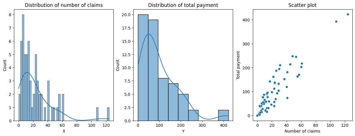
fig, (ax1, ax2, ax3) = plt.subplots(1, 3, figsize=(15, 5))
ax1.set_title('Distribution of number of claims')
ax2.set_title('Distribution of total payment')
ax3.set_title('Scatter plot')

sns.histplot(df.X, bins=50, kde=True, ax=ax1)
sns.histplot(df.Y, kde=True, ax=ax2)
sns.scatterplot(x=df.X, y=df.Y, ax=ax3)

ax3.set_xlabel('Number of claims')
ax3.set_ylabel('Total payment')

Text(0, 0.5, 'Total payment')

As we can see, two outliers are present with value total payment around 400 and number of claims \([100; 120]\). In data analysis, outliers are observations that lie far away from the majority of the data points in a dataset. Outliers can be caused by measurement errors, data entry errors, or rare events that have a significant impact on the data.

In this case, these outliers seems to be rare events as they are following the distribution. We can keep them in our dataset as they provide value for the training of the model.

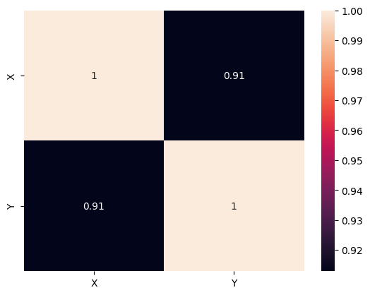
sns.heatmap(df.corr(), annot=True)

<Axes: >

Plotting the correlation heatmap is useful because it allows us to visualize the relationships between variables in a dataset. By examining the correlation matrix or heatmap, we can quickly identify which variables are positively or negatively correlated with each other, and how strongly they are correlated.

In this case, it is pretty obvious that the number of claims and total payment are highly correlated. The more a person makes a claim to the insurance, the more the total amount of money he will be paid is important.

Create Training Split

In machine learning, when training a model, we divide the dataset into subset. For the sake of comprehension let’s suppose we divide the data into two subsets: the training set and validation set. The training set is used to train the model, while the validation set is used to evaluate the model’s performance and tune its parameters.

The goal is to ensure that the model is able to generalize well to new, unseen data by testing its performance on a set of data that it has not been trained on.

data = df.to_numpy()
X = torch.from_numpy(data[:, 0]).float().unsqueeze(1)
y = torch.from_numpy(data[:, 1]).float().unsqueeze(1)
X_train, X_test, y_train, y_test = train_test_split(X, y, test_size=0.25, random_state=50)

Let’s explain this code line by line.
First, the data is loaded from a Pandas DataFrame into a Numpy array using the to_numpy() method.

Next, the input data and output data (groundtruths) are extracted from the numpy array and converted into PyTorch tensors using the torch.from_numpy() method. Specifically, the first column of the numpy array is used as the input data (X), and the second column is used as the groundtruth (y). The float() method is used to ensure that the data is converted to float data type, and the unsqueeze(1) method is used to reshape the data into the appropriate tensor shape.

Finally, the train_test_split() function from scikit-learn is used to split the data into training and testing sets, with a test size of 0.25 and a random state of 50 for reproducibility. The resulting variables (X_train, X_test, y_train, and y_test) are the input and output data for the machine learning model, which will be trained and evaluated using PyTorch.

The Least Square Method

The Least Squares method is a common approach for fitting a mathematical function to a set of data points by minimizing the sum of the squared differences between the predicted values of the function and the actual values in the dataset.

The method aims to find the best-fitting line or curve that describes the relationship between the variables in the data, by minimizing the difference between the predicted values of the model and the actual values in the dataset.

The Least Squares method can be formalized as the following optimization problem: \[\begin{align} \text{min} \sum (y_i - f(x_i)^2) \end{align}\]

The linear regression function f(x) is usually defined as: \[\begin{align} f(x) = b_0 + b_1x \end{align}\]

With the least square method, we find that: \[\begin{align} b_1 &= \frac{\text{Cov}(x, y)}{Var(x)} \\ b_1 &= \frac{\sum_i{(x_i - \mathbb{E}[x]) * (y_i - \mathbb{E}[y])}}{\sum_i{(x_i - \mathbb{E}[x])^2}}\\ b_0 &= \mathbb{E}[y] - b_1\mathbb{E}[x] \end{align}\]

The proof of this theorem is a convoluted process. In this article, we will assume these formulas as true. In this context, the esperance \(\mathbb{E}\) of a vector of random variables is its mean.

Now, let’s implement it in Pytorch with matrix calculus !

def linear_regression_1d(X, y):
    """Trains a linear regression on 1D data
    
    Args:
        X: A numpy array for the training samples
        y: A numpy array for the labels of each sample
    """
    # Compute esperance of x and y
    e_x = X.mean(dim=0)
    e_y = y.mean(dim=0)

    X_c = (X - e_x)
    
    # Compute covariance and variance
    covariance_xy = (X_c * (y - e_y)).sum(dim=0)
    variance_x = X_c.pow(2).sum(dim=0)

    # Divide covariance by variance
    b_1 = covariance_xy / variance_x
    
    # Get bias
    b_0 = e_y - b_1 * e_x.sum(dim=0)
    return b_0, b_1

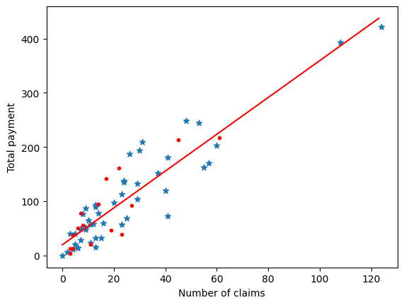
Display Regression Line

Let’s compute f(x) and visualize the regression line to see if it fits the data.

# Get the parameters of f(x), our linear regression function
b_0, b_1 = linear_regression_1d(X_train, y_train)

# Up to where to draw the regression line
x_upper_range = int(X.max())

# Every value of x to plot the regression line
x = torch.Tensor([int_ for int_ in range(0, x_upper_range)])

# Compute f(x)
y = b_0 + b_1 * x

plt.scatter(X_train, y_train, marker='*')
plt.scatter(X_test, y_test, marker='.', color='red')
plt.plot(x, y, color='red')

ax = plt.gca()
ax.set_xlabel('Number of claims')
ax.set_ylabel('Total payment')
plt.show()

As we discussed before, the inputs and the labels are very correlated so the regression line fits pretty well the distribution 🎉🎉🎉

Model Evaluation

In order to assess the performance of the model, we need to choose an approriate metric. We will use the Mean Squared Error (MSE), a commonly used metric to evaluate the performance of a machine learning model in predicting continuous variables. MSE is commonly defined as: \[\begin{align} \text{MSE} = \frac{1}{n} \sum_{i=0}^{n} (y - f(x))^2 \end{align}\]

Where y is the groundtruth and f(x) are the predicted values.

MSE is a popular choice as a performance metric is because it penalizes large errors more than small errors, due to the squaring of the difference between predicted and actual values.

err_train.abs().sum().pow(2) / y_train.shape[0]

tensor(36546.8125)

def mse(input_data, groundtruth, b_0, b_1):
    prediction = b_0 + b_1 * input_data
    error = groundtruth - prediction
    return error.T.mm(error) / len(groundtruth)


mse_train = mse(X_train, y_train, b_0, b_1)
mse_test = mse(X_test, y_test, b_0, b_1)

print(f'Train MSE:\t {mse_train.item()}')
print(f'Test MSE:\t {mse_test.item()}')

Train MSE:   1241.571533203125
Test MSE:    1279.6763916015625

The train and test MSE are close to each other. This is good news, it means that the model neither underfit nor overfit.